
Notice
Recent Posts
Recent Comments
Link
| 일 | 월 | 화 | 수 | 목 | 금 | 토 |
|---|---|---|---|---|---|---|
| 1 | 2 | 3 | 4 | |||
| 5 | 6 | 7 | 8 | 9 | 10 | 11 |
| 12 | 13 | 14 | 15 | 16 | 17 | 18 |
| 19 | 20 | 21 | 22 | 23 | 24 | 25 |
| 26 | 27 | 28 | 29 | 30 |
Tags
- 국비지원
- 대외활동
- 대중문화
- 미디어 콘텐츠
- 패스트캠퍼스부트캠프
- 지금 우리 학교는
- 유미의 세포들
- 패스트캠퍼스
- 이태원 클라쓰
- 부트캠프
- 대외활동 추천
- 미뮤엔토 에디터
- 현혹
- 이지스퍼블리싱
- 데이터분석
- 웹툰 원작
- 정년이
- 패스트캠퍼스데이터분석부트캠프
- BDA
- 데이터분석가
- 재혼황후
- 국비지원취업
- 딥러닝 스터디
- 미뮤엔토
- 딥러닝교과서
- 미유엔토
- 데이터분석취업
- 데이터분석부트캠프
- DOIT!
- 드라마
Archives
- Today
- Total
디지털 마케팅 LAB
BDA X 이지퍼블리싱 스터디 (4주차) 본문
pix2pix: 조건부 GAN을 사용한 이미지 대 이미지 변환
아래 과정에서는 입력 이미지에서 출력 이미지에 매핑하는 작업을 학습하는 pix2pix라는 cGAN(조건부 생성 적대 네트워크)을 구축하고 훈련하는 방법을 보여준다. pix2pix cGAN에서 입력 이미지에 대한 조건을 지정하고 해당 출력 이미지를 생성하는 방식이다.
TensorFlow 및 기타 라이브러리 가져오기
import tensorflow as tf

import os
import pathlib
import time
import datetime

from matplotlib import pyplot as plt
from IPython import display
데이터세트 로드하기
dataset_name = "facades"

_URL = f'http://efrosgans.eecs.berkeley.edu/pix2pix/datasets/{dataset_name}.tar.gz'

path_to_zip = tf.keras.utils.get_file(
    fname=f"{dataset_name}.tar.gz",
    origin=_URL,
    extract=True)

path_to_zip  = pathlib.Path(path_to_zip)

PATH = path_to_zip.parent/dataset_name

# 원본이미지는 256 x 256 이미지 2개가 포함된 256 x 512 크기
sample_image = tf.io.read_file(str(PATH / 'train/1.jpg'))
sample_image = tf.io.decode_jpeg(sample_image)
print(sample_image.shape)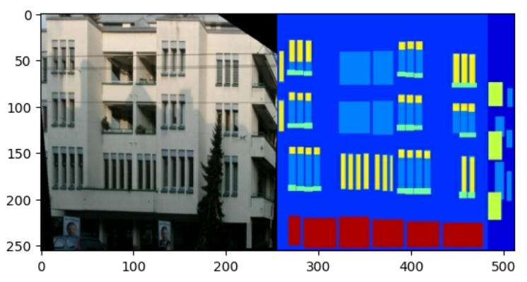
실제 건물 외관 이미지와 건축 레이블 이미지를 분리해야 하는데,
우선 이미지 파일을 로드하고 두 개의 이미지 텐서를 출력하는 함수를 정의한다.
def load(image_file):
  # Read and decode an image file to a uint8 tensor
  image = tf.io.read_file(image_file)
  image = tf.io.decode_jpeg(image)

  # Split each image tensor into two tensors:
  # - one with a real building facade image
  # - one with an architecture label image
  w = tf.shape(image)[1]
  w = w // 2
  input_image = image[:, w:, :]
  real_image = image[:, :w, :]

  # Convert both images to float32 tensors
  input_image = tf.cast(input_image, tf.float32)
  real_image = tf.cast(real_image, tf.float32)

  return input_image, real_image


# 입력(건축 레이블 이미지) 및 실제(건물 외관 사진) 이미지의 샘플을 플로팅한다.
inp, re = load(str(PATH / 'train/100.jpg'))
# Casting to int for matplotlib to display the images
plt.figure()
plt.imshow(inp / 255.0)
plt.figure()
plt.imshow(re / 255.0)
훈련 세트를 전처리하기 위해 랜덤 지터링과 미러링을 적용해야 한다.
# The facade training set consist of 400 images
BUFFER_SIZE = 400
# The batch size of 1 produced better results for the U-Net in the original pix2pix experiment
BATCH_SIZE = 1
# Each image is 256x256 in size
IMG_WIDTH = 256
IMG_HEIGHT = 256


# 각 256 x 256 이미지의 크기를 더 큰 높이와 너비(286 x 286)로 조정
def resize(input_image, real_image, height, width):
  input_image = tf.image.resize(input_image, [height, width],
                                method=tf.image.ResizeMethod.NEAREST_NEIGHBOR)
  real_image = tf.image.resize(real_image, [height, width],
                               method=tf.image.ResizeMethod.NEAREST_NEIGHBOR)

  return input_image, real_image


# 무작위로 다시 256 x 256으로 자른다.
def random_crop(input_image, real_image):
  stacked_image = tf.stack([input_image, real_image], axis=0)
  cropped_image = tf.image.random_crop(
      stacked_image, size=[2, IMG_HEIGHT, IMG_WIDTH, 3])

  return cropped_image[0], cropped_image[1]


# 이미지를 가로로 무작위로 뒤집는다.
def random_crop(input_image, real_image):
  stacked_image = tf.stack([input_image, real_image], axis=0)
  cropped_image = tf.image.random_crop(
      stacked_image, size=[2, IMG_HEIGHT, IMG_WIDTH, 3])

  return cropped_image[0], cropped_image[1]


# 이미지를 [-1, 1] 범위로 정규화
# Normalizing the images to [-1, 1]
def normalize(input_image, real_image):
  input_image = (input_image / 127.5) - 1
  real_image = (real_image / 127.5) - 1

  return input_image, real_image
@tf.function()
def random_jitter(input_image, real_image):
  # Resizing to 286x286
  input_image, real_image = resize(input_image, real_image, 286, 286)

  # Random cropping back to 256x256
  input_image, real_image = random_crop(input_image, real_image)

  if tf.random.uniform(()) > 0.5:
    # Random mirroring
    input_image = tf.image.flip_left_right(input_image)
    real_image = tf.image.flip_left_right(real_image)

  return input_image, real_image
훈련 및 테스트세트를 로드하고 사전 처리하는 몇 가지 도우미 함수를 정의
def load_image_train(image_file):
  input_image, real_image = load(image_file)
  input_image, real_image = random_jitter(input_image, real_image)
  input_image, real_image = normalize(input_image, real_image)

  return input_image, real_image


 def load_image_test(image_file):
  input_image, real_image = load(image_file)
  input_image, real_image = resize(input_image, real_image,
                                   IMG_HEIGHT, IMG_WIDTH)
  input_image, real_image = normalize(input_image, real_image)

return input_image, real_imagetf.data로 입력 파이프라인 구축하기
train_dataset = tf.data.Dataset.list_files(str(PATH / 'train/*.jpg'))
train_dataset = train_dataset.map(load_image_train,
                                  num_parallel_calls=tf.data.AUTOTUNE)
train_dataset = train_dataset.shuffle(BUFFER_SIZE)
train_dataset = train_dataset.batch(BATCH_SIZE)

try:
  test_dataset = tf.data.Dataset.list_files(str(PATH / 'test/*.jpg'))
except tf.errors.InvalidArgumentError:
  test_dataset = tf.data.Dataset.list_files(str(PATH / 'val/*.jpg'))
test_dataset = test_dataset.map(load_image_test)
test_dataset = test_dataset.batch(BATCH_SIZE)
생성기 구축하기
- 인코더의 각 블록: 컨볼루션 -> 배치 정규화 -> 누출이 있는 ReLU
- 디코더의 각 블록: 전치된 컨볼루션 -> 배치 정규화 -> 드롭아웃(처음 3개 블록에 적용됨) -> ReLU
- 인코더와 디코더 사이에는 건너뛰기 연결이 있다
인코더 정의
OUTPUT_CHANNELS = 3

def downsample(filters, size, apply_batchnorm=True):
  initializer = tf.random_normal_initializer(0., 0.02)

  result = tf.keras.Sequential()
  result.add(
      tf.keras.layers.Conv2D(filters, size, strides=2, padding='same',
                             kernel_initializer=initializer, use_bias=False))

  if apply_batchnorm:
    result.add(tf.keras.layers.BatchNormalization())

  result.add(tf.keras.layers.LeakyReLU())

  return result


down_model = downsample(3, 4)
down_result = down_model(tf.expand_dims(inp, 0))
print (down_result.shape)
디코더 정의
def upsample(filters, size, apply_dropout=False):
  initializer = tf.random_normal_initializer(0., 0.02)

  result = tf.keras.Sequential()
  result.add(
    tf.keras.layers.Conv2DTranspose(filters, size, strides=2,
                                    padding='same',
                                    kernel_initializer=initializer,
                                    use_bias=False))

  result.add(tf.keras.layers.BatchNormalization())

  if apply_dropout:
      result.add(tf.keras.layers.Dropout(0.5))

  result.add(tf.keras.layers.ReLU())

  return result


up_model = upsample(3, 4)
up_result = up_model(down_result)
print (up_result.shape)
다운샘플러와 업샘플러로 생성기를 정의
def Generator():
  inputs = tf.keras.layers.Input(shape=[256, 256, 3])

  down_stack = [
    downsample(64, 4, apply_batchnorm=False),  # (batch_size, 128, 128, 64)
    downsample(128, 4),  # (batch_size, 64, 64, 128)
    downsample(256, 4),  # (batch_size, 32, 32, 256)
    downsample(512, 4),  # (batch_size, 16, 16, 512)
    downsample(512, 4),  # (batch_size, 8, 8, 512)
    downsample(512, 4),  # (batch_size, 4, 4, 512)
    downsample(512, 4),  # (batch_size, 2, 2, 512)
    downsample(512, 4),  # (batch_size, 1, 1, 512)
  ]

  up_stack = [
    upsample(512, 4, apply_dropout=True),  # (batch_size, 2, 2, 1024)
    upsample(512, 4, apply_dropout=True),  # (batch_size, 4, 4, 1024)
    upsample(512, 4, apply_dropout=True),  # (batch_size, 8, 8, 1024)
    upsample(512, 4),  # (batch_size, 16, 16, 1024)
    upsample(256, 4),  # (batch_size, 32, 32, 512)
    upsample(128, 4),  # (batch_size, 64, 64, 256)
    upsample(64, 4),  # (batch_size, 128, 128, 128)
  ]

  initializer = tf.random_normal_initializer(0., 0.02)
  last = tf.keras.layers.Conv2DTranspose(OUTPUT_CHANNELS, 4,
                                         strides=2,
                                         padding='same',
                                         kernel_initializer=initializer,
                                         activation='tanh')  # (batch_size, 256, 256, 3)

  x = inputs

  # Downsampling through the model
  skips = []
  for down in down_stack:
    x = down(x)
    skips.append(x)

  skips = reversed(skips[:-1])

  # Upsampling and establishing the skip connections
  for up, skip in zip(up_stack, skips):
    x = up(x)
    x = tf.keras.layers.Concatenate()([x, skip])

  x = last(x)

  return tf.keras.Model(inputs=inputs, outputs=x)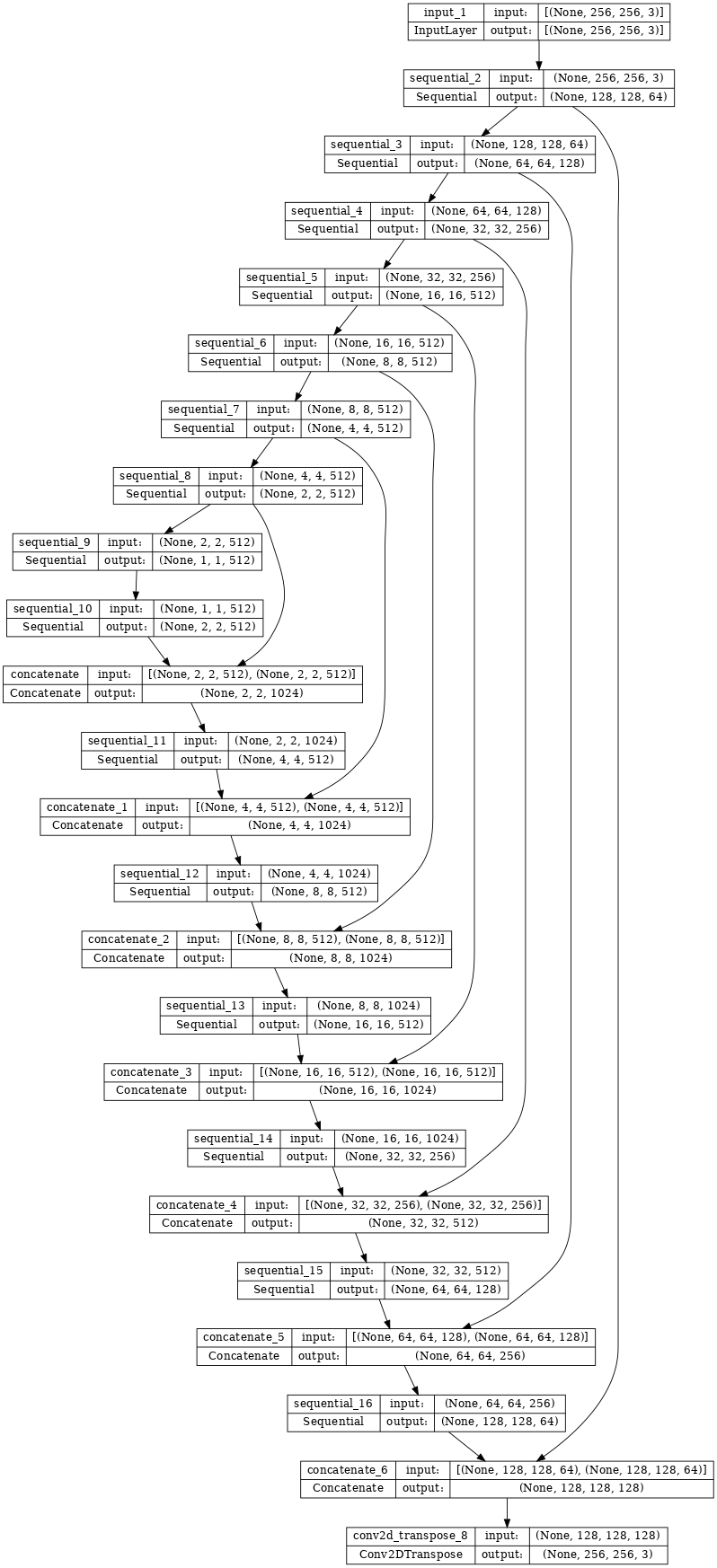
생성기 테스트
gen_output = generator(inp[tf.newaxis, ...], training=False)
plt.imshow(gen_output[0, ...])
생성기 손실 정의하기
GAN은 데이터에 적응하는 손실을 학습하는 반면 cGAN은 네트워크 출력 및 대상 이미지와 다른 가능한 구조에 불이익을 주는 구조화된 손실을 학습한다.
- 생성기 손실은 생성된 이미지와 1로 구성된 배열의 시그모이드 교차 엔트로피 손실이다.
- pix2pix 논문에는 생성된 이미지와 대상 이미지 간의 MAE(평균 절대 오차)인 L1 손실도 언급되어 있다.
- 이를 통해 생성된 이미지가 대상 이미지와 구조적으로 유사해질 수 있다.
- 총 생성기 손실을 계산하는 공식은 gan_loss + LAMBDA * l1_loss이고 여기서 LAMBDA = 100이다.
LAMBDA = 100

loss_object = tf.keras.losses.BinaryCrossentropy(from_logits=True)

def generator_loss(disc_generated_output, gen_output, target):
  gan_loss = loss_object(tf.ones_like(disc_generated_output), disc_generated_output)

  # Mean absolute error
  l1_loss = tf.reduce_mean(tf.abs(target - gen_output))

  total_gen_loss = gan_loss + (LAMBDA * l1_loss)

  return total_gen_loss, gan_loss, l1_loss
판별자 구축하기
pix2pix cGAN의 판별자는 컨볼루셔널 PatchGAN 분류기로, 각 이미지 패치가 실제인지 아닌지를 분류하려고 한다.
- 판별자의 각 블록: 컨볼루션 -> 배치 정규화 -> 누출이 있는 ReLU
- 마지막 레이어 이후의 출력 형상은 (batch_size, 30, 30, 1)이다.
- 출력의 각 30 x 30 이미지 패치는 입력 이미지의 70 x 70 부분을 분류한다.
- 판별자는 2개의 입력을 수신한다.
- 진짜로 분류해야 하는 입력 이미지 및 대상 이미지
- 가짜로 분류해야 하는 입력 이미지와 생성된 이미지(생성기의 출력)
- tf.concat([inp, tar], axis=-1)을 사용하여 이 2개의 입력을 함께 연결
def Discriminator():
  initializer = tf.random_normal_initializer(0., 0.02)

  inp = tf.keras.layers.Input(shape=[256, 256, 3], name='input_image')
  tar = tf.keras.layers.Input(shape=[256, 256, 3], name='target_image')

  x = tf.keras.layers.concatenate([inp, tar])  # (batch_size, 256, 256, channels*2)

  down1 = downsample(64, 4, False)(x)  # (batch_size, 128, 128, 64)
  down2 = downsample(128, 4)(down1)  # (batch_size, 64, 64, 128)
  down3 = downsample(256, 4)(down2)  # (batch_size, 32, 32, 256)

  zero_pad1 = tf.keras.layers.ZeroPadding2D()(down3)  # (batch_size, 34, 34, 256)
  conv = tf.keras.layers.Conv2D(512, 4, strides=1,
                                kernel_initializer=initializer,
                                use_bias=False)(zero_pad1)  # (batch_size, 31, 31, 512)

  batchnorm1 = tf.keras.layers.BatchNormalization()(conv)

  leaky_relu = tf.keras.layers.LeakyReLU()(batchnorm1)

  zero_pad2 = tf.keras.layers.ZeroPadding2D()(leaky_relu)  # (batch_size, 33, 33, 512)

  last = tf.keras.layers.Conv2D(1, 4, strides=1,
                                kernel_initializer=initializer)(zero_pad2)  # (batch_size, 30, 30, 1)

  return tf.keras.Model(inputs=[inp, tar], outputs=last)
판별자 테스트
disc_out = discriminator([inp[tf.newaxis, ...], gen_output], training=False)
plt.imshow(disc_out[0, ..., -1], vmin=-20, vmax=20, cmap='RdBu_r')
plt.colorbar()
판별자 손실 정의하기
- discriminator_loss 함수는 진짜 이미지와 생성된 이미지의 두 입력을 받는다.
- real_loss는 진짜 이미지 및 1의 배열(실제 이미지이기 때문에)의 시그모이드 교차 엔트로피 손실이다.
- generated_loss는 생성된 이미지 및 0의 배열(가짜 이미지이기 때문에)의 시그모이드 교차 엔트로피 손실이다.
- total_loss는 real_loss와 generated_loss의 합계이다.
def discriminator_loss(disc_real_output, disc_generated_output):
  real_loss = loss_object(tf.ones_like(disc_real_output), disc_real_output)

  generated_loss = loss_object(tf.zeros_like(disc_generated_output), disc_generated_output)

  total_disc_loss = real_loss + generated_loss

  return total_disc_loss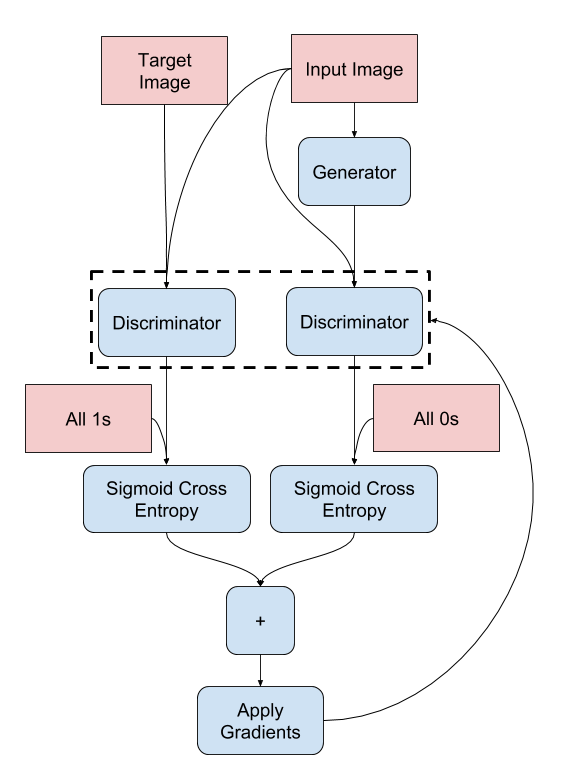
옵티마이저 및 체크포인트 세이버 정의하기
generator_optimizer = tf.keras.optimizers.Adam(2e-4, beta_1=0.5)
discriminator_optimizer = tf.keras.optimizers.Adam(2e-4, beta_1=0.5)

checkpoint_dir = './training_checkpoints'
checkpoint_prefix = os.path.join(checkpoint_dir, "ckpt")
checkpoint = tf.train.Checkpoint(generator_optimizer=generator_optimizer,
                                 discriminator_optimizer=discriminator_optimizer,
                                 generator=generator,
                                 discriminator=discriminator)
이미지 생성하기
훈련 중에 일부 이미지를 플롯하는 함수를 작성
- 테스트세트에서 생성기로 이미지를 전달
- 그러면 생성기가 입력 이미지를 출력으로 변환
- 마지막 단계는 예측을 플로팅하는 것
def generate_images(model, test_input, tar):
  prediction = model(test_input, training=True)
  plt.figure(figsize=(15, 15))

  display_list = [test_input[0], tar[0], prediction[0]]
  title = ['Input Image', 'Ground Truth', 'Predicted Image']

  for i in range(3):
    plt.subplot(1, 3, i+1)
    plt.title(title[i])
    # Getting the pixel values in the [0, 1] range to plot.
    plt.imshow(display_list[i] * 0.5 + 0.5)
    plt.axis('off')
  plt.show()


# 함수 테스트
for example_input, example_target in test_dataset.take(1):
  generate_images(generator, example_input, example_target)
훈련하기
- 각 예제 입력에 대해 출력을 생성
- 판별자는 input_image 및 생성된 이미지를 첫 번째 입력으로 받는다. 두 번째 입력은 input_image와 target_image이다.
- 다음으로 생성기와 판별자 손실을 계산
- 그런 다음 생성기와 판별자 변수(입력) 모두에 대한 손실 기울기를 계산하고 이를 옵티마이저에 적용
- 마지막으로 TensorBoard에 손실을 기록
log_dir="logs/"

summary_writer = tf.summary.create_file_writer(
  log_dir + "fit/" + datetime.datetime.now().strftime("%Y%m%d-%H%M%S"))


@tf.function
def train_step(input_image, target, step):
  with tf.GradientTape() as gen_tape, tf.GradientTape() as disc_tape:
    gen_output = generator(input_image, training=True)

    disc_real_output = discriminator([input_image, target], training=True)
    disc_generated_output = discriminator([input_image, gen_output], training=True)

    gen_total_loss, gen_gan_loss, gen_l1_loss = generator_loss(disc_generated_output, gen_output, target)
    disc_loss = discriminator_loss(disc_real_output, disc_generated_output)

  generator_gradients = gen_tape.gradient(gen_total_loss,
                                          generator.trainable_variables)
  discriminator_gradients = disc_tape.gradient(disc_loss,
                                               discriminator.trainable_variables)

  generator_optimizer.apply_gradients(zip(generator_gradients,
                                          generator.trainable_variables))
  discriminator_optimizer.apply_gradients(zip(discriminator_gradients,
                                              discriminator.trainable_variables))

  with summary_writer.as_default():
    tf.summary.scalar('gen_total_loss', gen_total_loss, step=step//1000)
    tf.summary.scalar('gen_gan_loss', gen_gan_loss, step=step//1000)
    tf.summary.scalar('gen_l1_loss', gen_l1_loss, step=step//1000)
    tf.summary.scalar('disc_loss', disc_loss, step=step//1000)
실제 훈련 루프
def fit(train_ds, test_ds, steps):
  example_input, example_target = next(iter(test_ds.take(1)))
  start = time.time()

  for step, (input_image, target) in train_ds.repeat().take(steps).enumerate():
    if (step) % 1000 == 0:
      display.clear_output(wait=True)

      if step != 0:
        print(f'Time taken for 1000 steps: {time.time()-start:.2f} sec\n')

      start = time.time()

      generate_images(generator, example_input, example_target)
      print(f"Step: {step//1000}k")

    train_step(input_image, target, step)

    # Training step
    if (step+1) % 10 == 0:
      print('.', end='', flush=True)


    # Save (checkpoint) the model every 5k steps
    if (step + 1) % 5000 == 0:
      checkpoint.save(file_prefix=checkpoint_prefix)
훈련 루프 실행
fit(train_dataset, test_dataset, steps=40000)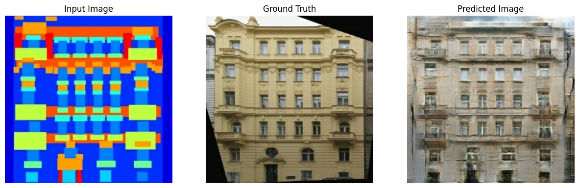
'BDA 딥러닝 easystudy' 카테고리의 다른 글
| BDA X 이지퍼블리싱 스터디 (3주차) (0) | 2023.05.29 |
|---|---|
| BDA X 이지퍼블리싱 스터디 (1주차) (0) | 2023.05.15 |
'BDA 딥러닝 easystudy' Related Articles
more
